TensorFlow - Local Response Normalization(LRN)（局所的応答正規化）

参考：theanoで局所コントラスト正規化(Local Contrast Normalization)を使う

正規化の方法にはいろいろあり、代表的なものを挙げると Global Contrast Normalization(GCN) Local Contrast Normalization(LCN) Local Response Normalization(LRN) ZCA whitening Local mean subtraction CNN内の正規化層としては、LCNやらLRNが使われる。 LCNはその名の通り、特徴マップの局所領域内でコントラストを正規化する。この処理は一つの特徴マップ内で完結するので、すべての特徴マップに対して独立して行う。対してLRNでは、同一位置における異なる特徴マップ間で正規化する。どちらもいくつかのハイパーパラメータはあるが、学習の対象となるパラメータはないので、誤差伝播が容易に可能である。

参考：theanoでLocal Response Normalization(LRN)を使う

LRNは端的に述べると、「同一位置(ピクセル)において複数の特徴マップ間で正規化する」ということだそうだ。元の論文にも書いてあるが、LRNは”brightness normalization”であり、LCNのように輝度の平均を減算して0にしないことがミソらしい。

[mathjax] $$\displaystyle bi {x,y}=a i{x,y}/ \left( k+\alpha \sum^{min(N-1,i+\frac{n}{2})}{j=max(0,i-\frac{n}{2})} (a j{x,y})2 \right)^\beta $$

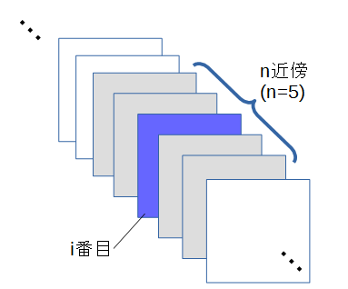
k, n, α, βがパラメータである ${a^i_{x,y}}$ はi番目の特徴マップの(x,y)のピクセルを、Nは特徴マップの総数を表す。 summationの部分は、「i番目の特徴マップに対して、n近傍の特徴マップの二乗和をとる」という意味である。

参考：tf.nn.local_response_normalization(input, depth_radius=None, bias=None, alpha=None, beta=None, name=None)

Local Response Normalization. The 4-D input tensor is treated as a 3-D array of 1-D vectors (along the last dimension), and each vector is normalized independently. Within a given vector, each component is divided by the weighted, squared sum of inputs within depth_radius. In detail,

翻訳結果

4次元入力テンソルは、（最後の次元に沿って）1次元ベクトルの3次元配列として扱われ、各ベクトルは独立して正規化されます。所与のベクトル内で、各成分は、depth_radius内の入力の加重二乗和で除算される。

sqr_sum[a, b, c, d] =
    sum(input[a, b, c, d - depth_radius : d + depth_radius + 1] ** 2)
output = input / (bias + alpha * sqr_sum) ** beta

使用例

norm1 = tf.nn.lrn(pool1, 4, bias=1.0, alpha=0.001 / 9.0, beta=0.75, name='norm1')

Python3で関数をつくってみる

def lrn(input, depth_radius, bias, alpha, beta):
    input_t = input.transpose([2, 0, 1])
    sqr_sum = np.zeros(input_t.shape)
    for i in range(input_t.shape[0]):
        start_idx = i - depth_radius
        if start_idx < 0: start_idx = 0
        end_idx = i + depth_radius + 1
        sqr_sum[i] = sum(input_t[start_idx : end_idx] ** 2)
    return (input_t / (bias + alpha * sqr_sum) ** beta).transpose(1, 2, 0)

使ってみる

import tensorflow as tf
import numpy as np
from PIL import Image

input = np.array([
    [
        [230,230,230],[210,210,210],[190,190,190],[170,170,170],[150,150,150]
    ],
    [
        [230,230,230],[210,210,210],[190,190,190],[170,170,170],[150,150,150]
    ],
    [
        [230,230,230],[210,210,210],[190,190,190],[170,170,170],[150,150,150]
    ],
    [
        [230,230,230],[210,210,210],[190,190,190],[170,170,170],[150,150,150]
    ],
    [
        [230,230,230],[210,210,210],[190,190,190],[170,170,170],[150,150,150]
    ],
])

depth_radius = 2
bias = 1.0
alpha = 0.001 / 9.0
beta = 0.75

def lrn(input, depth_radius, bias, alpha, beta):
    input_t = input.transpose([2, 0, 1])
    sqr_sum = np.zeros(input_t.shape)
    for i in range(input_t.shape[0]):
        start_idx = i - depth_radius
        if start_idx < 0: start_idx = 0
        end_idx = i + depth_radius + 1
        sqr_sum[i] = sum(input_t[start_idx : end_idx] ** 2)
    return (input_t / (bias + alpha * sqr_sum) ** beta).transpose(1, 2, 0)

output = lrn(input, depth_radius, bias, alpha, beta)
print(output)
Image.fromarray(np.uint8(output)).save('./img/lrn.jpg')

結果

[[[ 25.64542621  25.64542621  25.64542621]
  [ 26.62530279  26.62530279  26.62530279]
  [ 27.69886502  27.69886502  27.69886502]
  [ 28.8700044   28.8700044   28.8700044 ]
  [ 30.13193797  30.13193797  30.13193797]]

 [[ 25.64542621  25.64542621  25.64542621]
  [ 26.62530279  26.62530279  26.62530279]
  [ 27.69886502  27.69886502  27.69886502]
  [ 28.8700044   28.8700044   28.8700044 ]
  [ 30.13193797  30.13193797  30.13193797]]

 [[ 25.64542621  25.64542621  25.64542621]
  [ 26.62530279  26.62530279  26.62530279]
  [ 27.69886502  27.69886502  27.69886502]
  [ 28.8700044   28.8700044   28.8700044 ]
  [ 30.13193797  30.13193797  30.13193797]]

 [[ 25.64542621  25.64542621  25.64542621]
  [ 26.62530279  26.62530279  26.62530279]
  [ 27.69886502  27.69886502  27.69886502]
  [ 28.8700044   28.8700044   28.8700044 ]
  [ 30.13193797  30.13193797  30.13193797]]

 [[ 25.64542621  25.64542621  25.64542621]
  [ 26.62530279  26.62530279  26.62530279]
  [ 27.69886502  27.69886502  27.69886502]
  [ 28.8700044   28.8700044   28.8700044 ]
  [ 30.13193797  30.13193797  30.13193797]]]

tf.nn.lrnを使ってみる

コード

import tensorflow as tf
import numpy as np
from PIL import Image

input = np.array([
    [
        [230,230,230],[210,210,210],[190,190,190],[170,170,170],[150,150,150]
    ],
    [
        [230,230,230],[210,210,210],[190,190,190],[170,170,170],[150,150,150]
    ],
    [
        [230,230,230],[210,210,210],[190,190,190],[170,170,170],[150,150,150]
    ],
    [
        [230,230,230],[210,210,210],[190,190,190],[170,170,170],[150,150,150]
    ],
    [
        [230,230,230],[210,210,210],[190,190,190],[170,170,170],[150,150,150]
    ],
])

depth_radius = 2
bias = 1.0
alpha = 0.001 / 9.0
beta = 0.75

input_for_tf = np.zeros([1, input.shape[0], input.shape[1], input.shape[2]])
input_for_tf[0] = input
output2 = tf.nn.lrn(input_for_tf, depth_radius, bias=bias, alpha=alpha, beta=beta)
with tf.Session() as sess:
    out = sess.run(output2)
    print(out)
    Image.fromarray(np.uint8(out[0])).show()

結果

[[[[ 25.64542389  25.64542389  25.64542389]
   [ 26.62529945  26.62529945  26.62529945]
   [ 27.6988678   27.6988678   27.6988678 ]
   [ 28.87000465  28.87000465  28.87000465]
   [ 30.13193893  30.13193893  30.13193893]]

  [[ 25.64542389  25.64542389  25.64542389]
   [ 26.62529945  26.62529945  26.62529945]
   [ 27.6988678   27.6988678   27.6988678 ]
   [ 28.87000465  28.87000465  28.87000465]
   [ 30.13193893  30.13193893  30.13193893]]

  [[ 25.64542389  25.64542389  25.64542389]
   [ 26.62529945  26.62529945  26.62529945]
   [ 27.6988678   27.6988678   27.6988678 ]
   [ 28.87000465  28.87000465  28.87000465]
   [ 30.13193893  30.13193893  30.13193893]]

  [[ 25.64542389  25.64542389  25.64542389]
   [ 26.62529945  26.62529945  26.62529945]
   [ 27.6988678   27.6988678   27.6988678 ]
   [ 28.87000465  28.87000465  28.87000465]
   [ 30.13193893  30.13193893  30.13193893]]

  [[ 25.64542389  25.64542389  25.64542389]
   [ 26.62529945  26.62529945  26.62529945]
   [ 27.6988678   27.6988678   27.6988678 ]
   [ 28.87000465  28.87000465  28.87000465]
   [ 30.13193893  30.13193893  30.13193893]]]]

おーほぼほぼ同じだ。適当な別の配列でも試してみよう。

適当な配列でも試してみる

適当な配列

input = np.zeros([1, 5, 5, 3])
num = 1
for h in range(5):
    for w in range(5):
        for c in range(3):
            input[0][h][w][c] = num
            num += 1

結果

[[[[  1.   2.   3.]
   [  4.   5.   6.]
   [  7.   8.   9.]
   [ 10.  11.  12.]
   [ 13.  14.  15.]]

  [[ 16.  17.  18.]
   [ 19.  20.  21.]
   [ 22.  23.  24.]
   [ 25.  26.  27.]
   [ 28.  29.  30.]]

  [[ 31.  32.  33.]
   [ 34.  35.  36.]
   [ 37.  38.  39.]
   [ 40.  41.  42.]
   [ 43.  44.  45.]]

  [[ 46.  47.  48.]
   [ 49.  50.  51.]
   [ 52.  53.  54.]
   [ 55.  56.  57.]
   [ 58.  59.  60.]]

  [[ 61.  62.  63.]
   [ 64.  65.  66.]
   [ 67.  68.  69.]
   [ 70.  71.  72.]
   [ 73.  74.  75.]]]]

自作関数の結果

[[[  0.99883492   1.99766984   2.99650476]
  [  3.97452398   4.96815498   5.96178597]
  [  6.88892644   7.87305879   8.85719114]
  [  9.70624045  10.6768645   11.64748854]
  [ 12.39542092  13.34891484  14.30240875]]

 [[ 14.93127874  15.86448366  16.79768858]
  [ 17.29503693  18.20530203  19.11556713]
  [ 19.47436707  20.35956557  21.24476407]
  [ 21.46299164  22.32151131  23.18003097]
  [ 23.25997335  24.09068669  24.92140002]]

 [[ 24.86882105  25.67104108  26.47326112]
  [ 26.29652922  27.06995655  27.84338388]
  [ 27.55264319  28.29730922  29.04197525]
  [ 28.64841279  29.36462311  30.08083343]
  [ 29.59606986  30.28435055  30.97263125]]

 [[ 30.40824252  31.06929128  31.73034003]
  [ 31.09750348  31.7321464   32.36678933]
  [ 31.67603931  32.28519391  32.89434852]
  [ 32.15542323  32.74006729  33.32471135]
  [ 32.54647174  33.10761781  33.66876387]]

 [[ 32.85916694  33.39784181  33.93651668]
  [ 33.10262795  33.61985651  34.13708507]
  [ 33.28511771  33.78191052  34.27870332]
  [ 33.41407404  33.89141795  34.36876187]
  [ 33.49615612  33.95500757  34.41385903]]]

tf.nn.lrnの結果

[[[[  0.99883491   1.99766982   2.99650478]
   [  3.97452402   4.96815491   5.96178627]
   [  6.88892651   7.8730588    8.85719109]
   [  9.70624065  10.67686462  11.64748859]
   [ 12.39542103  13.34891415  14.30240822]]

  [[ 14.93127823  15.86448288  16.79768753]
   [ 17.29503632  18.20530128  19.11556625]
   [ 19.47436714  20.35956573  21.24476433]
   [ 21.46299171  22.32151222  23.18003082]
   [ 23.25997543  24.09068871  24.92140198]]

  [[ 24.86882019  25.67103958  26.47325897]
   [ 26.29652977  27.06995773  27.8433857 ]
   [ 27.55264282  28.29730988  29.04197502]
   [ 28.6484127   29.36462212  30.08083344]
   [ 29.59606934  30.28435135  30.97263145]]

  [[ 30.40824318  31.06929207  31.73034096]
   [ 31.09750175  31.73214531  32.36678696]
   [ 31.67603874  32.2851944   32.89434814]
   [ 32.15542221  32.74006653  33.32471085]
   [ 32.54647446  33.10762024  33.66876602]]

  [[ 32.85916519  33.39783859  33.93651581]
   [ 33.1026268   33.61985397  34.13708496]
   [ 33.2851181   33.78191376  34.2787056 ]
   [ 33.41407394  33.89141846  34.36876297]
   [ 33.49615479  33.95500946  34.41386032]]]]

ほぼ同じ。

大きい写真にLRNをしてみて結果をみてみる

画像はこれです。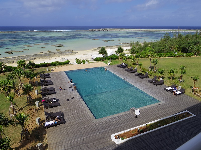

コード

import tensorflow as tf
import numpy as np
from PIL import Image

fpath = './img/sample_pic.jpg'
jpg = tf.read_file(fpath)
img = tf.image.decode_jpeg(jpg, channels=3)
input = tf.cast(tf.reshape(img, [1, 600, 800, 3]), dtype=tf.float32)

depth_radius = 2
bias = 1.0
alpha = 0.001 / 9.0
beta = 0.75

output = tf.nn.lrn(input, depth_radius, bias=bias, alpha=alpha, beta=beta)
with tf.Session() as sess:
    out = sess.run(output)
    print(out)
    Image.fromarray(np.uint8(out[0])).save('.・img/lrn_tf.jpg')

結果

これをCNNに入れ込むと効果が高まるって気づいた人すごいっす。